Class start delayed tomorrow

The University has delayed the start of classes tomorrow (Feb. 29th) until 10:30am.  That means we will not meet at 8:30.  Enjoy the extra sleep.

Solubility. {AGAIN?!?!}

When we talked about solubility, we said it was a dynamic process.  "Dynamic process" is super-secret science code for equilibrium.  If we want to think about solubility in its most generic terms, it is the reaction:

"ionic solid" ↔ "component ions"

Since pure solids do not appear in equilibrium constant expressions, the equilibrium constant for this type of reaction is just the product of the concentrations of the component ions, and is called a solubility product constant, with the symbol K_sp.  Although K_sp refers to a specific type of reaction, it's just another equilibrium constant so it follows all the same rules and has the same meaning as any other equilibrium constant.
For a specific example, let's consider the "insoluble" salt calcium sulfate.  Writing a K_sp-type chemical equation for calcium sulfate:

CaSO₄(s) ↔ Ca²⁺(aq) + SO₄^2-(aq)

K_sp = [Ca²⁺]_eq[SO₄^2-]_eq

"Insoluble" salts have reactant-favored K_sp's,
If we think about making a precipitate rather than dissolving a salt, we might think of a reaction like:

Ca(NO₃)₂(aq) + K₂SO₄(aq) ↔ CaSO₄(s) + 2 KNO₃(aq)

Equilibrium is really all about the chemical processes that are happening, not all the random fluff that might also be included like catalysts or spectator ions.  This means that we can always think about the net-ionic equation for a process at equilibrium rather than the full-molecular or full-ionic equation.  In fact, we can often completely eliminate terms from the equilibrium constant expression by using a net-ionic equation.  For the calcium sulfate equilibrium above, the full-ionic and net-ionic equation is:

Ca²⁺(aq) + 2 NO₃^-1(aq) + 2 K⁺(aq) + SO₄^2-(aq)  ↔  CaSO₄(s) + 2 K⁺(aq) + 2 NO₃^-1(aq)

Ca²⁺(aq) + SO₄^2-(aq)  ↔  CaSO₄(s)

That's the reverse of the K_sp equation for dissolving calcium sulfate, so we can manipulate the equilibrium constant expression and value to use in this situation.

Simplifying Approximations:
There are a couple approximations or assumptions that can make many of our equilibrium calculations a little easier to deal with.  These assumptions are usually valid for problems where the equilibrium is either quite strongly reactant-favored or quite strongly product-favored.  For very reactant-favored equilibria, we can assume that the change in concentration of reactants is small enough to be negligible.  For strongly product-favored equilibria, we can often treat the problem more like a limiting reactant/theoretical yield problem.  These approximations can be the only way to solve some of the higher order polynomials that come up fairly often in equilibrium calculations.

Correction from class:
As I said a few days ago, equilibrium problems are the places I am most like to get myself in trouble when I make things up during class.  I had a little "oops" today in class with the initial concentrations of the lead and sulfate stock solutions.  The set-up should have been 50.0mL of 1.0M solutions.  All the concentrations (and moles) in the equilibrium tables were fine if this stock concentration is used.

Manipulating equilibrium constants

What happens when we change the written form of a chemical reaction that describes an equilibrium?  This is usually necessary when we're looking at reaction mechanisms or other stepwise processes.

Multiplying a reaction:
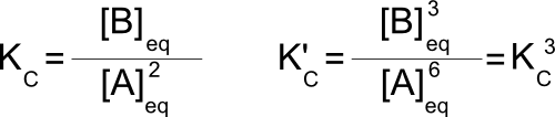
Consider the reaction 2A↔B with K=4.  We can multiply that reaction by 3 to get the reaction 6A↔3B.  Fundamentally, this is the same reaction and the same process, but what about the equilibrium constant?  Writing out the equilibrium constants for both reactions:

So if K = 4, K' = 4³ = 64

Changing direction:
If we reverse a chemical reaction, we once again have to adjust the equilibrium constant.  Changing 2A↔B to B↔2A means that we are changing the identity of reactants and product.  This means that the concentrations that used to be in the numerator of the equilibrium constant are now in the denominator and vice versa.  Mathematically, this has the effect of inverting the value of the equilibrium constant.  If K = 4 for 2A↔B, then K"=1/4 for B↔2A.

Multipart/Multistep:
For a multistep process, the equilibrium position of each step will affect the overall equilibrium of the system.  This is in contrast to kinetics where the rate law of the overall process relies only upon the rate law of the slowest step.  For a stepwise process, the equilibrium constant for the overall process is equal to the product of the individual steps.

Manipulating Equilibrium

Because equilibrium is a dynamic, thermodynamic process, there are a number of things we can do to "fiddle with" equilibrium systems.  Perhaps the most significant conceptual tool we have at our disposal is LeChatelier's Principle.  {Side note: To the francophones in the audience, I believe the "a" in "LeChatelier" is supposed to have a little hat on it...}
When a system at equilibrium experiences a stress, the position of that equilibrium will shift to relieve the stress (as much as is possible).
What's stress?  The most common type of stress we're likely to see in chemical reactions is adding or removing a reactant or product.  Let's think about the simple equilibrium reaction 2A↔B.  The equilibrium constant is:

If we add a little extra "A" to the reaction after equilibrium has been established (a stress), the reaction will have to shift toward the products to re-establish equilibrium.  If we look at the reaction quotient, Q, for a reaction, we can evaluate whether a system is at equilibrium, and if it is not, what direction the system has to shift to reach equilibrium.  The reaction quotient has the same mathematical form as the equilibrium constant; if Q if less than K, then there are too many reactants in the system and it must shift toward products.  If Q is greater than K, then there are too many products and the system must shift toward reactants.

Kinetics Experiments - The Nuts and Bolts

Last week in lab we performed a kinetics experiment in which we observed the iodination of acetone. For those of you who may be curious, there were a number of things that went into the planning of that experiment that are required to make it work as smoothly as it did. There is a certain art to experimental design, but it is all firmly rooted in the science that is being observed. For the kinetics of the iodination of acetone, the experimental design considerations are (in my opinion) fascinating, largely because they all make very good sense and can be understood with a Gen-Chem-level of knowledge.

1. Relative concentrations of the reactants. Some of you may have noticed that the concentration of the iodine was very much less than the concentration of the other reagents. This was not an accident. First, since we were observing the color of the solution and that color was due to the iodine, the concentration of iodine had to be high enough to be easily observable but low enough to react in a reasonable amount of time. In addition to this very practical consideration, there is a chemical reason for the concentrations used. The rate of a chemical reaction is dependent upon the concentration of the reactants. As “good” scientists, we always want to design our experiments in such a way that only one variable is changing. If, for example, the concentration of iodine was 1M and the concentration of acetone was also 1M, then as the iodine concentration changed (and affected the rate of the reaction), the acetone concentration would also change and would also affect the rate of the reaction. Although this data could be mathematically interpreted, it would be much more convenient if only one of the concentrations was changing during the reaction. Is this possible? Of course not. Iodine cannot disappear unless it reacts with acetone (in this reaction). BUT, we can make it seemlike the acetone concentration is not changing by making the initial concentration of acetone SO high, that the change will be very small, indeed “negligible”, compared to the change in the iodine concentration. To put some numbers to it, if the initial concentration of iodine is 5mM and the initial concentration of acetone is 1.000M and the reaction is allowed to proceed, when all of the iodine has reacted, the final concentration of acetone would be 0.995M. Yes, the concentration has changed, but it has changed by only 0.5%. This means that the change in rate caused by the change in concentration of acetone can be ignored. The reaction (and reaction rate) will observe the rate law order with respect to iodine only.
2. Limits of the Spec-20s. When we did the experiment, we said that the sample did not have to be put in the spectrometer until most of the color had faded. If anyone put their samples in the Spec-20 immediately, you might have noticed that the Spec-20 was unable to read the absorbance of the solution until most of the iodine color faded. This can be explained by thinking about the nature of “absorbance”. Absorbance is a logarithmic scale related to percent transmittance. An absorbance of “0” is equivalent to a percent transmittance of 100%. If the percent transmittance drops to 10%, the absorbance is “1”, which means 90% of the light that is shining on the sample is being absorbed. If the absorbance climbs to “2”, it means that only 1% of the incident light is getting through the sample (99% is absorbed). An absorbance of “3” means only 0.1% of the light is getting through. As we can see, increasing absorbance ver quickly decreases the amount of light getting through the sample. This brings us to the limits of the detector we are using. It can pretty easily discern the difference between 5% of the light being absorbed and 85% of the light being absorbed, but it's less reliable when trying to distinguish 97.8% absorbed and 98.5% absorbed. It is usually best practice to design experiments so the absorbances used are ~1.5 or less. If the absorbance is too high, the data will either get very “noisy”, or will just be abnormally low, making trends that should be linear appear curved.
3. Aggregation of solutes. This probably wouldn't have been a big problem in our iodination of acetone experiment, but Beer's Law assumes that the solute particles are separate and independent in solution. If the concentration of colored solute is relatively high, it's possible that the colored solute particles will start to interact in a way that will make them absorb differently than if they were truly separate and independent in solution. This is often solved by addressing the instrument limits mentioned in #2; if the sample is diluted sufficiently bring to the absorbance down below ~1.5, it is usually dilute enough to avoid interactions between solute particles.

There are other considerations, but these are the big ones that often come up in experimental design for kinetics experiments and any experiment where we are observing color using a spectrometer. For most of our experiments, we set things up behind the scenes to minimize or eliminate these problems, but I hope that some of you were curious enough to wonder why the experiment was set up the way it was.

See you in the morning.

Equilibrium is Organization!!

The key to equilibrium problems is almost always figuring out the best way to organize the data presented in the problem or experiment.  This is most often done by putting together a table.  Consider the following problem.

0.80mols NF₃(g) and 0.60mols O₂(g) are combined in a 1.00L vessel and allowed to reach equilibrium. At equilibrium, the concentration of NF₃(g) is found to be 0.30M. What is the value of the equilibrium constant for this reaction?
Write a balanced chemical equation:

2 NF₃(g) + O₂(g) ↔ 2 NO(g) + 3 F₂(g)

Set up a table to organize the data from the problem:

	2 NF3(g) +	O2(g) ↔	2 NO(g) +	3 F2(g)
[ ]initial	0.80 M	0.60 M	0 M	0 M
Δ[ ]	- 2x	- x	+ 2x M	+ 3x M
[ ]equil	(0.80-2x) M	(0.60-x) M	2x M	3x M

Write an expression for the equilibrium constant:

Plug in values from the table:

Determine "x" from the problem.  We are told that [NF3]eq=0.30M, and we see in the table that [NF3]eq=(0.80-2x), so:

0.30 = 0.80-2x

x = 0.25

Plugging in:

K = 3.4

This equilibrium is (very slightly) product-favored.

Practice, practice, practice...

Enter equilibrium

The steady state approximation applies to kinetic systems, but if we think about the nature of chemical reactions, we can say that all chemical reactions are microscopically reversible.  For the simple reaction A↔B

If we assume that the forward and reverse reaction both represent elementary steps, we can write rate law expressions for each direction:

Rate_forward = k_forward[A]₀

Rate_reverse = k_reverse[B]₀

After some time has passed, the rate of the forward reaction will be equal to the rate of the reverse reaction.

Rate_forward = Rate_reverse
k_forward[A]₀ = k_reverse[B]₀     

Rearranging to group constants and concentrations, we get the expression for the equilibrium constant.

K_eq = [products]_eq / [reactants]_eq  

If [products]_eq = [reactants]_eq, then K_eq = 1 and the reaction does not favor products or reactants.  If the equilibrium is product-favored, the the value of K_eq will be larger than 1; if the equilibrium is reactant-favored, the the value of K_eq will be less than 1 but still positive.

Mechanisms

The mechanism for a chemical reaction is described by the rate law.  Mechanisms describe the collisional events that allow a reaction to occur and must obey 3 rules.

1. A mechanism must be composed of elementary steps/reactions.
2. The elementary steps of a mechanism, when added together, must yield the overall reaction
3. The observed rate law for the overall reaction must be consistent with the rate law for the slowest step

Elementary steps are the collisions that occur in a reaction.  Thinking about the probability of a collision, we can simplify the picture a little bit because it is extremely unlikely that more than 2 particles will collide with the proper orientation and energy to react.  This means that all elementary steps are either unimolecular or bimolecular.  {Yes, termolecular elementary steps are possible, but they're rarely significant contributors so we will ignore them for now.}
Once we have this series of elementary steps, what do we do with them?  Because elementary steps describe collisions at the molecular level, we can write rate laws for each of the elementary steps based only upon the balanced reaction of the elementary step.  Since doubling the number of any molecule will double the probability of a collision (the rate), the elementary steps are first order with respect to each reacting molecule.
Rates are determined by the activation energy of a step or an overall process; the higher the activation energy, the slower the rate.  For a series of steps, whichever step has the highest activation energy will determine (or limit) the rate for the entire process, so it is known as the Rate Determining (or Limiting) Step, the RDS (or RLS).  With a little algebra, we can wrassle the rate law of the RDS into a form that looks like the observed rate law.  The rate law expression for the overall process shown below, A + B + D→E, is

Rate_obs = k_obs[A]₀^x[B]₀^y[D]₀^z

If the first step is RDS, we can write the rate law expression for the first step:

Rate₁=k₁[A]₀¹[B]₀^y

This rate law, looks just like the observed rate law if the reaction is first order with respect to [A] and [B], so if the first step is RDS, this is a pretty straight-forward problem with minimal algebraic wrasslin'.

For the second step RDS, we have to use a steady state approximation to make the rate law "consistent with" the observed rate law.  The rate law for the second step is:

Rate₂=k₂[C]₀¹[D]₀¹

But [C] does not appear in the overall observed rate law expression, so we have to figure out a way to make this expression "consistent with" the observed rate law for the overall process.  If most of "C+D" has quite a bit of energy, but not quite enough to get over the C+D→E hump, it probably has enough energy to go backwards and return to "A+B".  This means we can define another rate law, this time for the reverse of step 1, C+D→A+B:

Rate_-1=k_-1[C]₀¹[D]₀¹

As the rxn A+B→C+D proceeds, eventually we will build up a concentration of "C+D" that will remain essentially constant throughout the reaction.  This is the "steady state".  When we reach this steady state, the rate of step 1 going forward (Rate₁) will be equal to the rate of step 1 in reverse (Rate_-1):

Rate₁ = Rate_-1

Which means that:

k₁[A]₀¹[B]₀¹ = k_-1[C]₀¹[D]₀¹

Now we can solve for  [C]₀¹ :

[C]₀¹ = {k₁/k_-1}[A]₀¹[B]₀¹/[D]₀¹

Now, we can plug the expression for  [C]₀¹ into the rate law expression for step 2:

Rate₂ =  k₂({k₁/k_-1}[A]₀¹[B]₀¹/[D]₀¹)[D]₀¹ = k_combined[A]₀¹[B]₀¹  

Note: Since "k₁", "k_-1", and "k₂" are constants, we can just lump them together into a single constant, in this case labelled "k_combined".

So if the second step is slow, the observed rate law should be first order w.r.t. [A] and [B], zero order w.r.t. [D].  Note that this is the same as the observed rate law expression if the first step is slow, so how can we distinguish between these two mechanisms?  Typically there would have to be something else observable in the reaction.  If step 2 is slow, then during the course of the reaction, we might expect to see a measurable concentration of "C" appear when the steady state is established and then disappear when the reaction is complete.  We might also be able to analyse the value of "k_observed" to see a difference, but that's often a bit more challenging than detecting an intermediate in the reactions.

Yikes, that one got a little long.  Have a good weekend.

Logarithms

Logarithms used to be extremely important.  With modern calculators, logarithms aren't quite as critical as they used to be, but they're still very useful in some cases.  There are a few definitions and identities that will help us out a bit, the most basic ones are:

log (10^x) = 10^{log x} = x

ln (e^x) = e^{ln x} = x

The following work for either common logs (log, base 10) or natural logs (ln, base "e"):

log (AB) = log A + log B

log (A/B) = log A - log B

log (A^B) = B log A

A little practice will help lock these in.  Good luck.

Integrated Rate Laws and Activation Energy

There's a new bit of OWL assignment posted, make sure you take a look.

Rate laws can tell us a lot about a reaction, but a simple rate law doesn't do a great job of telling us how fast or slow a reaction really is.  In order to incorporate a time component, we can integrate the rate law expressions.  The integrated rate laws (IRLs) give us a way to monitor the way concentrations change over time.

0^th Order IRL → [A]_t = -kt + [A]₀

1^st Order IRL → ln[A]_t = -kt + ln[A]₀

2^nd Order IRL → {1/[A]_t} = kt + {1/[A]₀}

IRLs can also be used to determine the order of a reaction with respect to a given reactant.  All of the IRLs listed above are equations of lines.  If we plot [A]_t vs. t and the result is a straight line, then the process must be 0^th order w.r.t. [A].  Likewise, a linear plot of ln[A]_t vs. t implies a 1^st order process, and a linear plot of {1/[A]_t} vs. t implies a 2^nd order process.

Why do reactions have the rates they do?  This is a function of the amount of energy required to make a reaction occur.  Recall from Collision Theory that collisions must occur and those collisions must be oriented and energetic.  The energy required to get a reaction started is the activation energy, E_a.  Activation energy is described by the Arrhenius equation:

k = A exp(-E_a/RT)

where:

k = rate law constant

A = frequency factor

E_a = activation energy

R = universal gas constant, 8.314 J/mol.K

T = temperature in units of Kelvin

Although this is an elegant little bit of mathematics, it's not the most useful form of the Arrhenius equation.  If 2 sets of conditions are known, we can set up a ratio of the Arrhenius equation for each run and ultimately find that:

ln(k₁/k₂) = (E_a/R)({1/T₂} - {1/T₁})

The comparative form works well, but it has a notable flaw.  We have to assume that both of the points of data that we have a quite good and accurate.  Hopefully this is the case, but it might not be, leading to error.  If we want to average out some of that error, we can do another transformation of the Arrhenius equation to form a line:

ln(k) = (-E_a/R)(1/T) + ln(A)

Friday we'll look more closely at activation energy and what it means in terms of reaction mechanisms.

Rate Laws

We can calculate the instantaneous rate for any point in a concentrations vs. time experiment, but the only really unique and important one is the initial instantaneous rate.  The initial rate of a reaction is described by a rate law.  The initial rate of a chemical reaction is proportional to the initial concentration of all the reactants raised to some power.  To remove the proportionality, we can add a constant, the rate law constant.

Rate₀ = k [reactant]₀^x

We can write a rate law expression for any chemical reaction as long as we know the reactants.  For example, for the generic reaction:

aA + bB → cC + dD

The rate law expression is

Rate₀ = k[A]₀^x[B]₀^y

If we think about this rate law expression, there seem to be a LOT of variables present.  We can determine the value of a number of those variables if we design our experiments thoughtfully.  Let's look at a specific example.
For the reaction of NO₂(g) with Cl₂(g), we have performed the following experiment: [NO₂]₀ = 1.228M, [Cl₂]₀ = 1.316M, Rate₀ = 2.881x10^{-3 M}/_min.  The rate law expression for this reaction is:

Rate₀ = k [NO₂]₀^x[Cl₂]₀^y

Notice that we don't really need to know the products or the balanced chemical equation to write out the rate law expression.  That doesn't mean we don't have to practice balancing chemical equation, keep on practicing!!  Plugging the numbers in to the rate law expression:

(2.881x10^{-3 M}/_min) = k (1.228M)^x(1.316M)^y

That's still 3 variables, so we need (mathematically) more equations to help us solve them.  We could just randomly start mixing reactants together, but if we're deliberate in our planning, we can make our jobs a little easier.  As good scientists, we try to change one 1 variable at a time whenever we're doing an experiment.  Why?  Because then if the result changes, we know it has to be caused by the variable we changed.  In this case, we can set up another experiment, and let's change the initial concentration of NO₂ but hold the initial concentration of Cl₂ constant.  For our second run: [NO₂]₀ = 2.456M, [Cl₂]₀ = 1.316M, Rate₀ = 1.152x10^{-2 M}/_min.  Plugging in to the rate law expression again, we get:

(1.152x10^{-2 M}/_min) = k (2.456M)^x(1.316M)^y

Let's get a little mathematical here... if these two equalities are valid (which they are), then their ratio is also a valid equality.  Bam.  Cancelling out everything that can cancel, we're left with the simplified expression:

(1/4) = (1/2)^x

x = 2

Therefore, the reaction is second order with respect to [NO₂]₀.

Kinetics, at an average rate...

Kinetics is the study of the rates and mechanisms/pathways of chemical reactions.  Most of kinetics can be understood by probability and the 3 points of Collision Theory: For a chemical reaction to occur: 1) Collisions between reactant particles must occur; 2) The collisions must be energetic enough to allow reaction; 3) The colliding particles must be oriented in a way that gives the desired reaction.  The probabilities is Collision Theory are affected by changes in temperature and concentration/pressure.

Rates can be expressed in a number of ways, but for most chemical systems, the rate is equal to the change in concentration over the change in time.  When that change in time is (relatively) long, we have an average rate.  Average rates can be either in terms of consumption of a reactant or production of a product.  The mathematical formality of "change in concentration" requires a negative sign on rates of consumption.  Rates of consumption or production are related to the stoichiometric coefficients in the balances chemical equation that is being observed and can be unified as a rate of reaction.

A significant disadvantage of average rates is that they change depending upon the time period being measured.  To more accurately estimate the rate of a reaction, we should use smaller time periods.  Taken to the extreme, we can calculate an instantaneous rate at any point during a reaction.  Of all the instantaneous rates for a given reaction, the only important or unique instantaneous rate is the very first one, the initial instantanous rate of the reaction.

On Friday, we'll continue with kinetics.  You will very likely NOT get your exams back on Friday.  A number of things came up today (and continue tomorrow) that will make it difficult to get exams back on Friday.  I will have them done over the weekend and will return them first thing Monday morning.  Sorry for the delay.